

Sentiment analysis - London restaurants reviews
Overview
The goal of this project is to analyze the customers' sentiments based on Yelp restaurant reviews.
This type of analysis is known as a part of NLP tasks and highly used for business purposes, such as online marketing automation, measurement of product's users exeperience and etc.
We will use London restaurant reviews, scrapped from Yelp website.
In this particular task we will follow the steps below to complete end-to-end machine learning project:
- Import necessary libraries;
- Data gathering and cleansing;
- Explanatory analysis;
- Models building and result comparison;
- Making prediction.
The closing section sums up the project results and aprovides the further improvement recommendations.
Libraries import
First we will use Beautifulsoup library to scrap data. Next we store reviews with corresponding ratings to pandas frame and visualize with wordcloud amd matplotlib. Finally we import scikit-learn modules for models building and evaluation.
Python code
"""
- importing urllib2, BeautifulSoup and requests for yelp web-scrapping
- pandas, matplotlib, numpy - for data manipulation

"""
import urllib2
from bs4 import BeautifulSoup
import requests
import csv
import pandas as pd
import matplotlib.pyplot as plt
import numpy as np

"""
- libraries for working with text and visualizing output

"""
from collections import Counter
import nltk
from wordcloud import WordCloud
from nltk import FreqDist # get word count
from nltk.tokenize import word_tokenize # tokenize the sentences by word

"""
- model building and measure performance
- parametres are estimated with grid search

"""
from sklearn import metrics
from sklearn.utils import shuffle # shuffle data before learning curve plotting
from sklearn.model_selection import train_test_split

from sklearn.linear_model import LogisticRegression
from sklearn.metrics import accuracy_score
from sklearn.model_selection import learning_curve
import scikitplot as skplt

from sklearn.model_selection import GridSearchCV
from sklearn.ensemble import AdaBoostClassifier
from sklearn.tree import DecisionTreeClassifier
Data preparation
The restaurants listed on Yelp wibsite and used for reviews collecting.
restaurants = [
'https://www.yelp.com/biz/hide-london?start=',
'https://www.yelp.com/biz/a-wong-london?start=',
'https://www.yelp.com/biz/restaurant-gordon-ramsay-london-3?start=',
'https://www.yelp.com/biz/dinner-by-heston-blumenthal-london?start=',
'https://www.yelp.com/biz/the-breakfast-club-london-3?start=',
'https://www.yelp.com/biz/five-guys-london-23?start=',
'https://www.yelp.com/biz/kowloon-london?osq=Kowloon+Restaurant?start=',
'https://www.yelp.com/biz/cubana-london?start=',
'https://www.yelp.com/biz/pizza-east-london?start=',
'https://www.yelp.com/biz/las-iguanas-london?start=',
'https://www.yelp.com/biz/mother-mash-london?start=',
'https://www.yelp.com/biz/shake-shack-covent-garden-london-4?start=',
'https://www.yelp.com/biz/meat-liquor-london?start=',
'https://www.yelp.com/biz/lupita-london-9?start=',
'https://www.yelp.com/biz/jamies-italian-covent-garden-london?start=']
Here we will create the empty lists for reviews and corresponding ratings. With each link from restaurants list opened we will iterate through the range of pages and scrap reviews data.
Python code
review_list=[]
rating_list=[]
pages=range(0,260,20)

# create a list of all pages for each restaurat
all_pages=[]

for url in restaurants:
   for page in pages:
       rest_page = url+str(page)
       all_pages.append(rest_page) # append the next page to list

"""
- open each link with urllib2
- read the content with Beautiful soup
- find corresponding review text and rating under 'div' calss on html page

"""

for link in all_pages:
   content = urllib2.urlopen(link)
   soup = BeautifulSoup(content, 'html.parser')

   for review in soup.findAll('div',{"class":"review-content"}):
       rating_list.append(review.div.div.div.get("title"))
       review_list.append(review.find('p').text)
Next we will initialize dataframe and add columns with both text and rating we scrapped on previous step.
Python code
reviews = pd.DataFrame()
reviews['rating'] = rating_list
reviews['rating'] = reviews['rating'].str[:3]
reviews['reviews'] = review_list

"""
- remove punctuation from sentences
- lead all words to a lower case
- convert rating to float and write into csv  to save results

"""
reviews['reviews_punctuation_free'] = reviews['reviews'].str.replace('[^\w\s]',' ') # used space, since some words can be merged
reviews['reviews_punctuation_free'] = reviews['reviews_punctuation_free'].str.lower()

reviews['rating'] = reviews['rating'].astype('float64')
reviews.to_csv('sent_reviews.csv', sep='\t', encoding='utf-8')
Assign sentiment classes
For each review in frame we assign the sentiment class in order to split the reviews on positive or negative and create a target label.
- rating = 4.0 and 5.0 --> class = 1
- rating < 2.0 --> class = 0
- rating = 3.0 --> do not include, neutral assessment
Python code
reviews = reviews[reviews['rating'] != 3.0]
reviews['sentiment'] = reviews['rating'].apply(lambda rating : +1 if rating >= 4.0 else 0)
# display how dataframe looks like
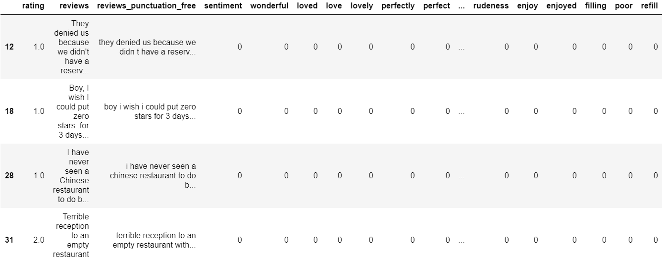
reviews.tail(10)
Explanatory analysis
Imbalance classes
Starting explanatory analysis with investigating balance classes we can plot the number of reviews assigned to each class.
Python code
plt.style.use('bmh') # set up matplotlib style

fig, ax = plt.subplots(figsize=(7,5))
reviews['sentiment'].value_counts().plot.bar()
ax.set_xlabel('sentiment')
ax.set_title('Sentiment classes')
Python code
# display the number of each class in percentage
(reviews['sentiment'].value_counts(normalize=True)*100).round(2)
1    78.07
0    21.93
Name: sentiment, dtype: float64
Bar chart above highlight significant imbalance classes with positive major class. One of the propriate ways to mitigate imbalance is to make the equal proportion for both classes. However, the obvious disadvantage of this approach leads to entire sample reduction.
Python code
"""
- split frame into parts based on positive/negarite sentiment
- undersample the major class to keep equal size for both
- create dataframe with balanced classes

"""
positive_frame = reviews[reviews['sentiment']==1]
negative_frame = reviews[reviews['sentiment']==0]

# estimate the size ratio
percentage = len(negative_frame)/float(len(positive_frame))
negative = negative_frame
positive = positive_frame.sample(frac=percentage) # use the same percentage
# append negative reviews sample to reduced positive frame
reviews_data = negative.append(positive)

print "Positive class ratio:", len(positive) / float(len(reviews_data))
print "Negative class ratio:", len(negative) / float(len(reviews_data))
print "Entire frame length:", len(reviews_data)
Positive class ratio: 0.5
Negative class ratio: 0.5
Entire frame length: 894
Words count and visualization
For each review perform transformation into string type and generate the cloud of words using Wordcloud() module.
Python code
text_pos=str() # initialize strig for positive  frame
for rev in positive_frame['reviews_punctuation_free']:
   rev=str(rev)
   text_pos = text_pos+rev

# create wordcloud object with text_pos as an argument
wordcloud = WordCloud(background_color='white', width=1600, height=800).generate(text_pos)
# plot as a figure
plt.figure(figsize=(12,8))

plt.imshow(wordcloud, interpolation = 'bilinear')
plt.axis('off')
plt.tight_layout(pad=0)
plt.show()
Next we complete the same procedure for negative reviews.
Python code
text_neg=str() # initialize strig for negative  frame
for word in negative_frame['reviews_punctuation_free']:
   word=str(word)
   text_neg = text_neg+word

wordcloud = WordCloud(background_color='white', width=1600, height=800).generate(text_neg)

plt.figure(figsize=(12,8))

plt.imshow(wordcloud, interpolation = 'bilinear')
plt.axis('off')
plt.tight_layout(pad=0)
plt.show()
As we can conclude from charts the most common words display neutral customers sentiments and gereral term (such as 'food', 'place', 'london' or 'order', 'pizza') rather than feelings or particular experience. Let's tokenize the words and sort them with respect of frequency.
Python code
"""
- create a token object as a list of words, count the occurence respectively using FreqDist() module
- display the frequency for number of words (250 in example)

"""

nltk.download('punkt')

from nltk import FreqDist # used later to plot and get count
from nltk.tokenize import word_tokenize # tokenizes our sentence by word

token = word_tokenize(text_pos)

fdist = FreqDist(token)

fdist.most_common(250)
Here are some words from tokenized list - note that the most frequent words have neutral sentiment.
[('the', 12530),
('and', 7823),
('a', 6438),
('i', 5877),
('to', 4624),
('was', 4117),
('of', 4014),
('it', 3675),
('in', 2903),
('is', 2552),
('for', 2512),
('with', 2324),
('you', 2100),
('but', 2009),
('we', 1983),
...
('recommend', 201),
('bar', 201),
('cake', 201),
('want', 199),
('being', 198),
('way', 197),
('ice', 197),
('ll', 196),
('loved', 196),
('over', 196),
('sweet', 196),
('who', 194),
('excellent', 193),
('pork', 193),
('off', 192),
('eat', 191),
('know', 191),
('gravy', 190),
('every', 189)
Then display frequency for negative cases:
Python code
token = word_tokenize(text_neg)
fdist = FreqDist(token)
fdist.most_common(250)
[('the', 3745),
('and', 2194),
('to', 2019),
('a', 1827),
('i', 1751),
('was', 1358),
('it', 1118),
('of', 1050),
('we', 892),
('in', 840),
('for', 793),
('that', 691),
...
('thing', 48),
('dirty', 48),
('bland', 48),
('couple', 48),
('okay', 47),
('decent', 47),
('star', 47),
('already', 46),
('put', 46),
('since', 46),
('doesn', 46),
('want', 45),
('little', 45)]
Model selection
Since the majority of words for both positive and negative samples represent neutral sentiment, the reasonable solution seemed to prepare the bunch of sensitive words as features to build the separating hyperplane and hit the better model performance.
Keywords selection
Collection of features represents both positive and negative customer's restaurant experience.
keywords = ['wonderful', 'loved', 'love', 'lovely', 'perfectly', 'perfect', 'disappointed', 'terrible', 'nasty',
           'recommend', 'delicious', 'served', 'dirty', 'amazing', 'excellent', 'good', 'friendly','tasty',
           'fantastic','happy', 'never', 'gross', 'decent', 'service', 'like', 'bad', 'rudeness', 'enjoy', 'enjoyed',
           'filling','poor', 'refill','awful', 'hungry', 'hate', 'hated']
Next we will estimate the count for the number of times the keyword occurs in the review. As a result of feature processing a single column for each word will be created.
Python code
# create a binary column for each word in 'reviews_punctuation_free' column
for i in keywords:
   reviews_data[i] = reviews_data['reviews_punctuation_free'].apply(lambda x : x.split().count(i))
reviews_data.head()
Train-test split
First, we make a split with 10% of test data. We will use this to make predictions later. Then, split rest of the data into a train-validation with 80% of training set and 20% of the data for the validation set.
Python code
"""
- split train_val and test data
- split train and validation
- create variables for features and label data

"""

train_val_data, test_data = train_test_split(reviews_data, test_size=0.1)
train_data, validation_data = train_test_split(train_val_data, test_size=0.2)

# display train, validation proportion
print 'Training sample   : %d' % len(train_data)
print 'Validation sample : %d' % len(validation_data)

feature_train = train_data[keywords]
sentiment_train = train_data['sentiment']

feature_val = validation_data[keywords]
sentiment_val = validation_data['sentiment']
Training sample   : 643
Validation sample : 161
Training simple model (regularization not included)
We start model building with simple logistic regression - we will fit model on train dataset and measure accuracy on validation.
Python code
"""
- since l2 is default penalty, we can take c as high value C=1e4
- C approaches 0 and cost function becomes standard error function

"""

simple_model = LogisticRegression(penalty = 'l2', C=1e4, random_state = 1)
simple_model.fit(feature_train, sentiment_train)
sentiment_pred = simple_model.predict(feature_val)
simple_score = accuracy_score(sentiment_val, sentiment_pred)

print 'Simple model accuracy validation: ' + str(round(simple_score, 3))
Simple model accuracy validation: 0.783
L2 regularization effects
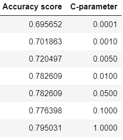
Then let's fit the model with different L2 regalarization parameters.
First, we are going to list the values of $λ = 1/c$ and fit the model with parametres $c$ - the inverse of regularization strength. Small value of c leads to strong regularization.
Python code
c_param = [0.0001, 0.001, 0.005, 0.01, 0.05, 0.1, 1] # range of c = 1/lambda coefficients
score_list = []

for c in c_param:
   model = LogisticRegression(penalty = 'l2', C = c,random_state = 1)
   model.fit(feature_train, sentiment_train)
   sentiment_pred = model.predict(feature_val)
   score = accuracy_score(sentiment_val, sentiment_pred)
   score_list.append(score)

"""
- represent the results of different regularization strength as dataframe

"""
scores = pd.DataFrame({'C-parameter': c_param, 'Accuracy score': score_list})

scores
Best-model coefficients
Next we going to show fit logistic regression model with best regularization parameter to shortlist the coefficient values. Recall the large coefficients values attest potential overfitting of model.
Python code
"""
- fit model with c = 0.05 as best performed on validation set
- create dataframe with coefficients of fitted model
"""
reg_model = LogisticRegression(penalty = 'l2', C = 0.05, random_state = 1)
reg_model.fit(feature_train, sentiment_train)
# concat the features list (keywords) and corresponding values
coefficients = pd.concat([pd.DataFrame(feature_train.columns),
pd.DataFrame(np.transpose(reg_model.coef_))],
axis = 1)
coefficients.columns = ['Feature', 'coefficients']
coefficients = coefficients.append({'Feature':'Intercept',
'coefficients':reg_model.intercept_[0]},
ignore_index=True)
coefficients.sort_values('coefficients', ascending=False)

Feature	       coefficients
delicious	0.753607
amazing	        0.618723
loved	        0.515113
perfect	        0.480637
excellent	0.415803
tasty	        0.362062
perfectly	0.352833
love	        0.305544
recommend	0.303009
happy	        0.301588
wonderful	0.258520
lovely	        0.257344
enjoy	        0.187139
enjoyed   	0.173547
friendly	0.130182
fantastic	0.116963
served	        0.073657
good	        0.070752
hated	        0.000000
Intercept      -0.064563
rudeness       -0.076226
filling	       -0.142474
service        -0.197804
hate	       -0.202412
hungry	       -0.204982
like	       -0.205757
poor	       -0.240060
never	       -0.248887
terrible       -0.267078
decent	       -0.280627
gross	       -0.292031
awful	       -0.293193
refill	       -0.308748
dirty	       -0.347450
nasty	       -0.366258
disappointed   -0.450833
bad	       -0.485633
Evaluating accuracy on test data
Python code
"""
- use .predict() method to make predictions
- calculate the accuracy score on test

"""
simple_pred = simple_model.predict(test_data[keywords])
simple_score = accuracy_score(test_data['sentiment'], simple_pred)

print 'Simple model accuray: ' + str(round(simple_score, 3))
Simple model accuracy: 0.822
Use the same method to calculate score for regularized model.
Python code
reg_pred = reg_model.predict(test_data[keywords])
reg_score = accuracy_score(test_data['sentiment'], reg_pred)

print 'Regularized model accuray: ' + str(round(reg_score, 3))
Regularized model accuracy: 0.833
Adaptive Boosting Classifier
To improve the performance of classification model we able to apply ensemble algorithm as a combinataion of weaker classification algorithms for each iteration $t = 1...T$ .
The common choice would be Adaptive Boosting algorithm evaluation. We will fit a model testing different parametres via search grid to approach the optimum.
Python code
"""
- first, we test the range of trees for descision classifier and learning rate
- establish a minimal number for internal node split = 5

"""
n_trees = range(10, 50, 5)
learning_rate = [0.0001, 0.001, 0.01, 0.1]
dtree = DecisionTreeClassifier(random_state = 1, min_samples_split=5) # create decision tree classifier object
adboost = AdaBoostClassifier(base_estimator=dtree)
"""
- additionally we will use two metrics for spliting a tree - gini and entropy criteria
- specify 3 folds cross-validation as a gridsearch parameter

"""

param = {'base_estimator__criterion' : ['gini', 'entropy'],
        'learning_rate': learning_rate,
         "n_estimators": n_trees}

grid_cv = GridSearchCV(adboost, param_grid=param, scoring = 'accuracy', cv=3)

grid_cv.fit(feature_train, sentiment_train)
GridSearchCV(cv=3, error_score='raise-deprecating',
      estimator=AdaBoostClassifier(algorithm='SAMME.R',
         base_estimator=DecisionTreeClassifier(class_weight=None, criterion='gini', max_depth=None,
           max_features=None, max_leaf_nodes=None,
           min_impurity_decrease=0.0, min_impurity_split=None,
           min_samples_leaf=1, min_samples_split=5,
           min_weight_fraction_leaf=0.0, presort=False, random_state=1,
           splitter='best'),
         learning_rate=1.0, n_estimators=50, random_state=None),
      fit_params=None, iid='warn', n_jobs=None,
      param_grid={'n_estimators': [10, 15, 20, 25, 30, 35, 40, 45], 'base_estimator__criterion': ['gini', 'entropy'], 'learning_rate': [0.0001, 0.001, 0.01, 0.1]},
      pre_dispatch='2*n_jobs', refit=True, return_train_score='warn',
      scoring='accuracy', verbose=0)
Show the best model score on validation and related parametres.
Python code
print round(grid_cv.best_score_,4)
print grid_cv.best_params_
0.7558
{'n_estimators': 45, 'base_estimator__criterion': 'entropy', 'learning_rate': 0.001}
Calculate predictions for AdaBoost and show accuracy on test data.
Python code
best_adboost = grid_cv.best_estimator_
predictions = best_adboost.predict(test_data[keywords])
round(metrics.accuracy_score(test_data['sentiment'], predictions),4)
0.7667
Learning curve
In order to illustrate the accuracy score change with respect to train-validation sample size, we will plot the learning curves for trained models.
Python code
"""
- return values from dataframe, suffle features and label
- define a function to evaluate learning curve on train size range
- print mean score on each train sample and plot curves for train and validation

"""

X=reviews_data[keywords].values
y=reviews_data['sentiment'].values
X_shuf, y_shuf = shuffle(X, y)

def plot_learning_curve(model):
   train_sizes, train_scores, test_scores = learning_curve(model, X_shuf, y_shuf, train_sizes=np.arange(0.1,1., 0.2),
                                                                      cv=3, scoring='accuracy')
   print 'Training sample size: ' + str(train_sizes)
   print 'Mean score for train samples: ' + str(train_scores.mean(axis = 1))
   print 'Mean score for test samples: ' + str(test_scores.mean(axis = 1))

   plt.figure(figsize=(9,7))
   plt.plot(train_sizes, train_scores.mean(axis = 1), 'b-', marker='o', label='train')
   plt.plot(train_sizes, test_scores.mean(axis = 1), '--', color='#af2c18', marker='o', label='validation')
   plt.ylim((0.0, 1.05))
   plt.legend(loc='upper right')
   plt.xlabel("training size", size=12)
   plt.ylabel("accuracy score", size=12)
plot_learning_curve(simple_model)
plt.title('Logistic regression - unregularized', size=15)
Training sample size: [ 59 178 298 417 536]
Mean score for train samples: [0.97175141 0.85580524 0.82997763 0.82014388 0.81156716]
Mean score for test samples: [0.68120805 0.75167785 0.76510067 0.76733781 0.79194631]
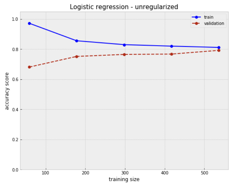
The accuracy on train sample goes down along with train sample increasing. On the other hand, validation score grows starting from 50 observations and gets flat reached sample size equals 250. However gap between train and validation doesn't seem significant.
Python code
plot_learning_curve(reg_model)
plt.title('Logistic regression - L2 regularized', size=15)
Training sample size: [ 59 178 298 417 536]
Mean score for train samples: [0.80225989 0.79213483 0.80425056 0.79776179 0.79850746]
Mean score for test samples: [0.67225951 0.72930649 0.75615213 0.76957494 0.78411633]
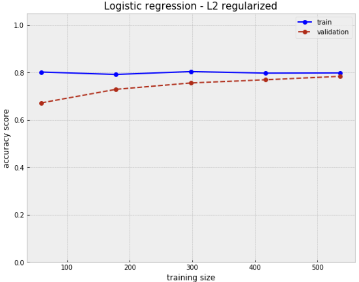
From learning curve above we see the regularization parameter for logistic regression slightly underfits the data compared to a simple regularization free model. The gap between train and validation remains small.
Python code
plot_learning_curve(best_adboost)
plt.title('Adaptive Boosting model', size=15)
Training sample size: [ 59 178 298 417 536]
Mean score for train samples: [0.98305085 0.91947566 0.92393736 0.91686651 0.91044776]
Mean score for test samples: [0.67337808 0.7147651  0.7393736  0.73378076 0.75391499]
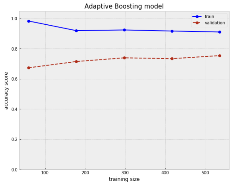
Despite the fact Adaboost models are not prone to overfitting, they tend to be sensitive to noisy data. The gap between train and validation seems more considerable, but keeps decreasing slightly with larger train sample.
Evaluating results on ROC curve
Finally, validate the results of models plotting ROC curve for each to illustrate graphically sensitivity and specificity for pairs with respect to decision threshold.
Python code
"""
- return the probabilities for binary classification
- plot receiver operating curve
"""
def roc_curve(model):
plt.figure(figsize=(9,7))
y_probs = model.predict_proba(test_data[keywords])
skplt.metrics.plot_roc(test_data['sentiment'], y_probs,
figsize=(9,7), title=None, cmap='Blues')
# plot ROC for simple regularization free model
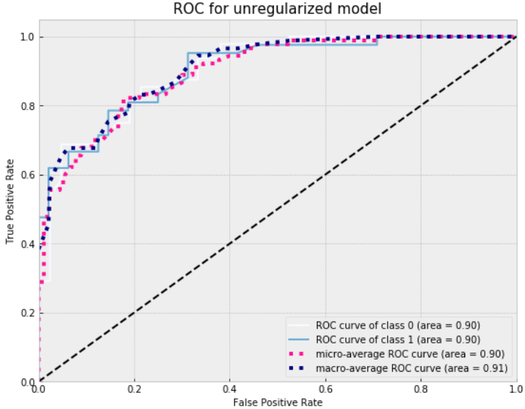
roc_curve(simple_model)
plt.title('ROC for unregularized model', size=15)
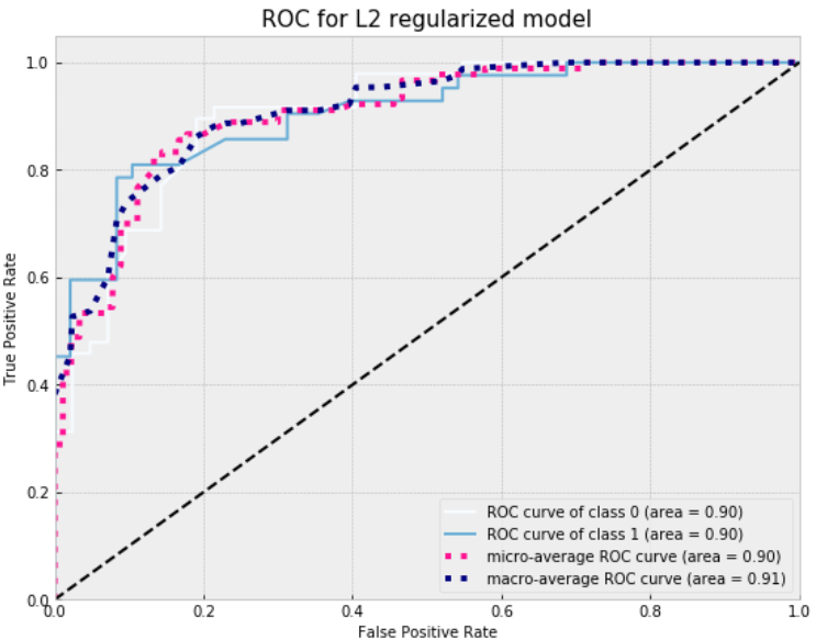
Plot ROC curve for L2 regularized model.
Finally plot ROC curve for AdaBoost.
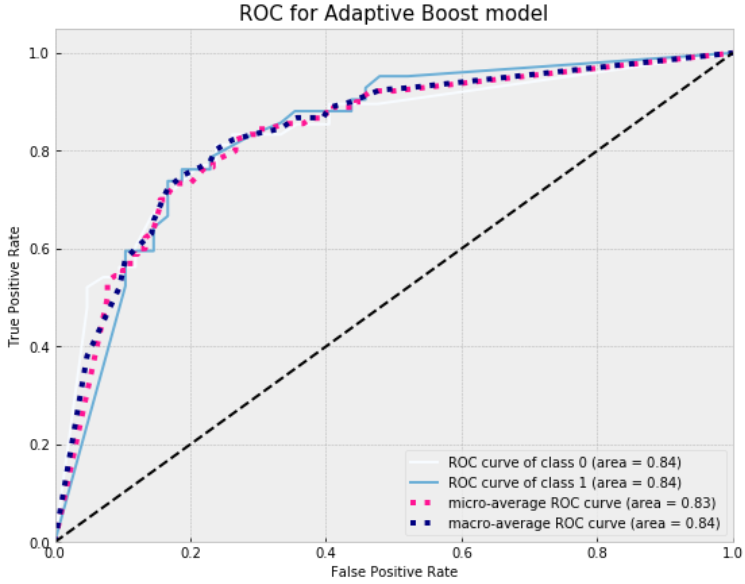
The charts above presents the highest overall accuracy and sensitivity/specificity tradeoff on test for regularized logistic model with parameter C=0.05. However, in our case simple and regularized model perform in similar way. The less accurate performance was shown by AdaBoost model, that could be explained by the fact of sensitivity to noisy data .
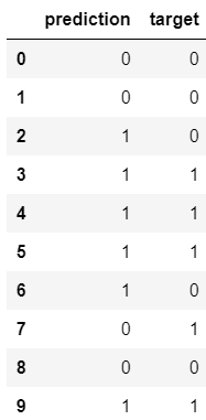
Best model predictions
Form the best model predictions as a dataframe and compare them with test labels.
Python code
"""
- create a dataframe object
- combine predictions with target on test, write to csv

"""
pred = pd.DataFrame()
target=list(test_data['sentiment'])
pred['prediction']=reg_pred
pred['target']=target

pred.to_csv('pred-target.csv', sep='\t', encoding='utf-8')
pred.head(10)
Further improvements
The next steps for reaching higher modeling performance can be taken in following directions:
- Lexical normalization:
- Characters repetition, elonged words handling;
- Reviews translation - train additional machine learning model to translate the sentences;
- Features engineering:
- Focus on words relationship, paired words influence;
- POS tagging use to identify the emotional tokens of content words;
- Use of lexicon-based algorithms, more orientated on semantic analysis and syntactic relationships.