
Spotify: Music Data retrieve and EDA
About Spotify
Originally found in Sweden, Spotify became one of the largest worldwide music streaming services. Since 2006 company has been growing its popularity and reached 87 million paying subscribers in November 2018. The large number of Spotify users allowed to create significant content database and retreive valuable patterns from tracks attributes.
For current project we used developers documentation and Web API to access music data, provided by platform. Full code in Jupyter notebook is available in repository
Data:
We will go through official documentation, using "Search" endpoint reference to collect data, includes:
- tracks metadata;
- artists' attributes;
- audio features.
Install libraries, API connection setting
Let's store data into panads data frame and import visualization libraries for explanatory analysis part.
Python code
import pandas as pd
import numpy as np
import seaborn as sns
import matplotlib.pyplot as plt
from collections import Counter
from wordcloud import WordCloud

%matplotlib inline
from pylab import rcParams

plt.style.use('bmh')

"""
- establish client credentials for authentification

"""
import spotipy
import spotipy.util as util
from spotipy.oauth2 import SpotifyClientCredentials
We access data with username and client id of application, registrated on developers page. Additionally we need to use token with scope, such as user library/playlist read/modify to retreive tracks and attributes.
Python code
"""
- we access data with username and client id of application, registrated
- import visualization libraries for explanatory analysis part

"""

username='XXXXXX' # Spotify username
scope = 'user-library-read playlist-modify-public playlist-read-private'
client_id='XXXXX' # app-redirect url
client_secret='XXXXXXXXX'

redirect_uri='http://localhost:8888/callback/' # Paste your Redirect URI here
client_credentials_manager = SpotifyClientCredentials(client_id=client_id, client_secret=client_secret)
sp = spotipy.Spotify(client_credentials_manager=client_credentials_manager)
token = util.prompt_for_user_token(username, scope, client_id, client_secret, redirect_uri)

if token:
   sp = spotipy.Spotify(auth=token)
else:
   print("Token is not accessible", username)
Part 1 - retrieve the tracks' list
On this stage we will retrieve tracks metadata: artist name, album name, track name, popularity, track id and write into data frame.
Python code
"""
- generate empty lists for related track's characteristics
- using sp.search() will iterate through 2018 tracks, appending items in lists

"""

artist_ids=[]
artist_names=[]
track_names=[]
track_ids=[]
popularity_score=[]

for i in range(0,10000,10):
   res=sp.search(q='year:2018', type='track', offset=i)
   for i, j in enumerate(res['tracks']['items']):
       artist_id = j['artists'][0]['id']
       artist_ids.append(artist_id)
       artist_name = j['artists'][0]['name']
       artist_names.append(artist_name)
       track_name = j['name']
       track_names.append(track_name)
       track_id = j['id']
       track_ids.append(track_id)
       track_popularity = j['popularity']
       popularity_score.append(track_popularity)
# create data frame with lists as columns
track_attributes = pd.DataFrame({'artist_ids':artist_ids, 'artist_names':artist_names, 'track_names':track_names, 'track_ids':track_ids, 'popularity_score':popularity_score})
Part 2 - retrieve the artists' genres
However Spotify documentation does not provide the way to look up the genres tags for selected tracks from database. Hence, we will use the same approach to get artists data using Spotify.search().
Python code
# create the lists for artists ids and genres tags
artist_ids_genres=[]
genres_all=[]

for i in range(0,10000,10):
   res_genres=sp.search(q='year:2018', type='artist', offset=i)
   for i, j in enumerate(res_genres['artists']['items']):
       artist_id_genre=j['id']
       artist_ids_genres.append(artist_id_genre)
       artist_genre=j['genres']
       genres_all.append(artist_genre)

# separate tags with comma
genres_list = [', '.join(x) for x in genres_all]
genres = pd.DataFrame({'artist_ids':artist_ids_genres, 'genres_all':genres_list})

genres.to_csv('genres.csv')
Part 3 - retrieve the tracks' features
Additionally we are going to retreive the attributes: energy, liveness, acousticness, instrumentalness, loudness, danceability and valence. Before writing into frame, its worth checking for 'None' values - otherwise, the error can be occured.
Python code
"""
- start with empty list - it will include the sets of all features
- check for None values
- write a list into dataframe

"""
features = []
for i in range(0,len(track_ids)):
   track=str(track_ids[i])
   audio_features = sp.audio_features(track)
   for track in audio_features:
       features.append(track)
# use list comprehension, leave elements that are not None
f = [feat for feat in features if feat is not None]
playlist_df = pd.DataFrame(f)
playlist_df.rename(columns={'id': 'track_ids'}, inplace=True)

playlist_df.head()
Part 4 - enitire dataframe collection
Finally we merge all collected dataframes in one to prepare for explanatory analysis.
Python code
"""
- start with empty list - it will include the sets of all features
- check for None values
- write a list into dataframe

"""
features = []
for i in range(0,len(track_ids)):
   track=str(track_ids[i])
   audio_features = sp.audio_features(track)
   for track in audio_features:
       features.append(track)
# use list comprehension, leave elements that are not None
f = [feat for feat in features if feat is not None]
playlist_df = pd.DataFrame(f)
playlist_df.rename(columns={'id': 'track_ids'}, inplace=True)

playlist_df.head()
Delete columns we don't need for analysis and check NaN values.
Python code
"""
- read from csv and and drop NaNs
- display the shape of frame

"""
df = pd.read_csv('tracks_data.csv', sep='\t', encoding='utf-8')
df.drop(['artist_ids', 'track_ids', 'analysis_url', 'track_href', 'uri', 'key', 'type', 'Unnamed: 0'], axis=1, inplace=True)

df.isna().any()
df.dropna(inplace=True)
df.to_csv('tracks_assignment.csv', sep='\t', encoding='utf-8')
print df.shape
df.head()
(1533, 16)
Explanatory data analysis
Audio fetaures exploration
We will start describing the dataframe and analysis of popularity score.
As per documentation, the score value ranges from 0 (least popular) to 100 (most popular) and primarily based on number of plays the track achieved.
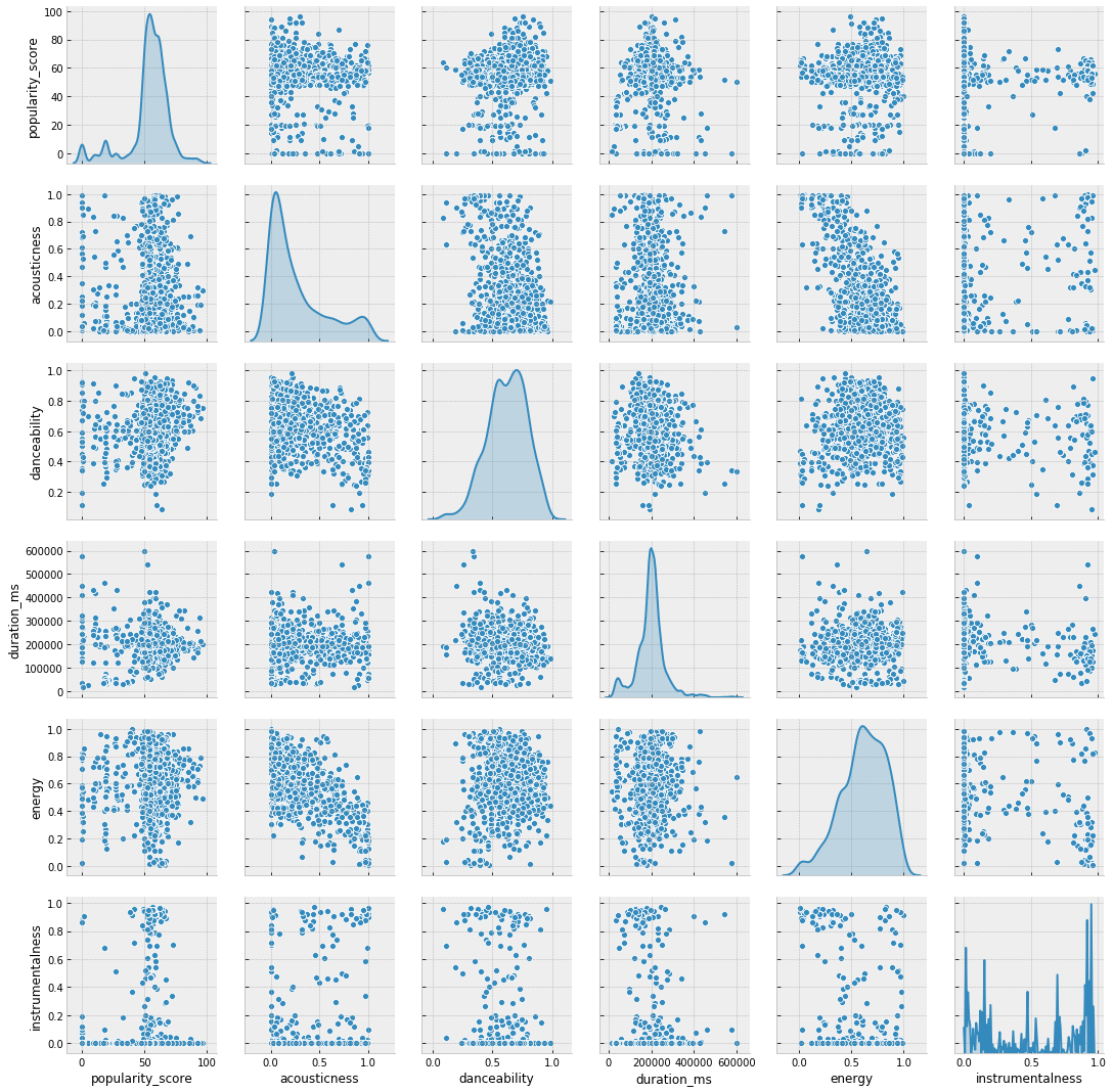
How does popularity score relate to other audio features? Is there any correlation between all variables?
Next we will visualize paired correlation between numerical variables.
Python code
"""
- with seaborn library display pairplots; add density plots on main diagonal

"""

scatter = sns.pairplot(df[['popularity_score', 'acousticness', 'danceability',
                          'duration_ms', 'energy', 'instrumentalness']], diag_kind="kde")
Python code
"""
- include popularity score in list to visulaize correlation between rest of variables

"""
scatter2 = sns.pairplot(df[['popularity_score',
                        'liveness', 'loudness', 'speechiness', 'tempo', 'valence']], diag_kind="kde")

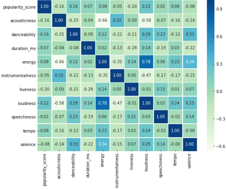
We see few features show high correlation on pairplots. Then, form a heatmap to summarize the correlation ratio.
Python code
"""
- estimate correlations in matrix form
- plot seaborn heatmap with annotation bar

"""

numeric=['popularity_score', 'acousticness', 'danceability',
        'duration_ms', 'energy', 'instrumentalness',
        'liveness', 'loudness', 'speechiness', 'tempo', 'valence']

matrix = df[numeric].corr()
y, x = plt.subplots(figsize=(9, 7))

heatmap = sns.heatmap(matrix, annot=True, fmt=".2f", linewidths=.5, cmap="GnBu")
plt.show()
To investigate the correlation for energy-loudness and energy-acousticness pairs we can build jointplots for each combination.
Python code
"""
- first, display jointplot
- add annotation bar to plot, specifying properties as 'arrowprops'

"""
# plot for energy-loudness pair
sns.jointplot(x="loudness", y="energy", data=df, kind="hex", height=4.5)

plt.annotate('Energy-loudness relation',
            xy=[0.1, 0.6],
            xytext=[1, 1.2],
            fontsize=14,
            arrowprops=dict(color='grey',
                            arrowstyle='simple',
                            shrinkA=4,
                            shrinkB=4))

# plot for energy-acousticness pair
sns.jointplot(x="acousticness", y="energy", data=df, kind="hex", height=4.5)


plt.annotate('Energy-acousticness relation',
            xy=[0.1, 0.6],
            xytext=[1, 1.2],
            fontsize=14,
            arrowprops=dict(color='grey',
                            arrowstyle='simple',
                            shrinkA=4,
                            shrinkB=4))
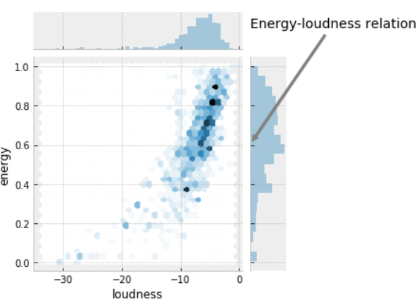
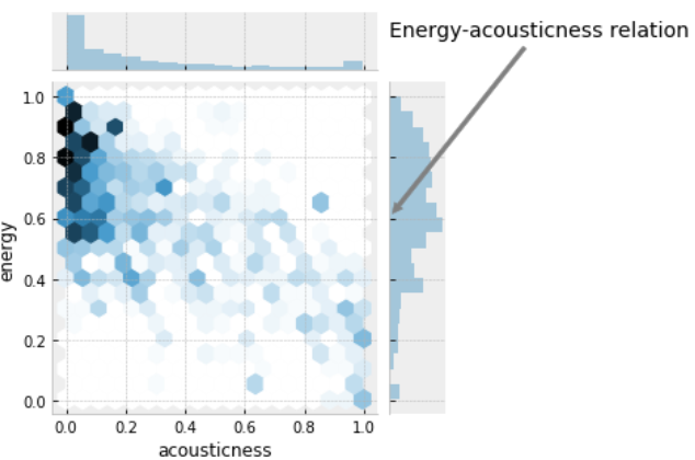
Paired charts shows the positive correlation character for energy and loudness, while energy-accousticness pair behaves in opposite way: energy goes down as acousticness rate increase.
Artist - Genre exploration
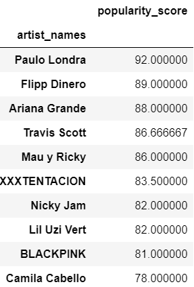
To continue with explanatory analysis we will summarize popularity score per artist and top 10 least and most popular artists from sample.
Python code
artist_df = pd.pivot_table(df, values='popularity_score', index=['artist_names'], aggfunc=np.mean)

artist_df.fillna(0, inplace=True)
# shortlist top 10 artist by popularity
artist_df=artist_df.sort_values(by=['popularity_score'], ascending=False)
artist_df.head(10)
Python code
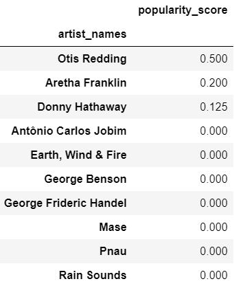
# shortlist 10 least popular
artist_df.tail(10)
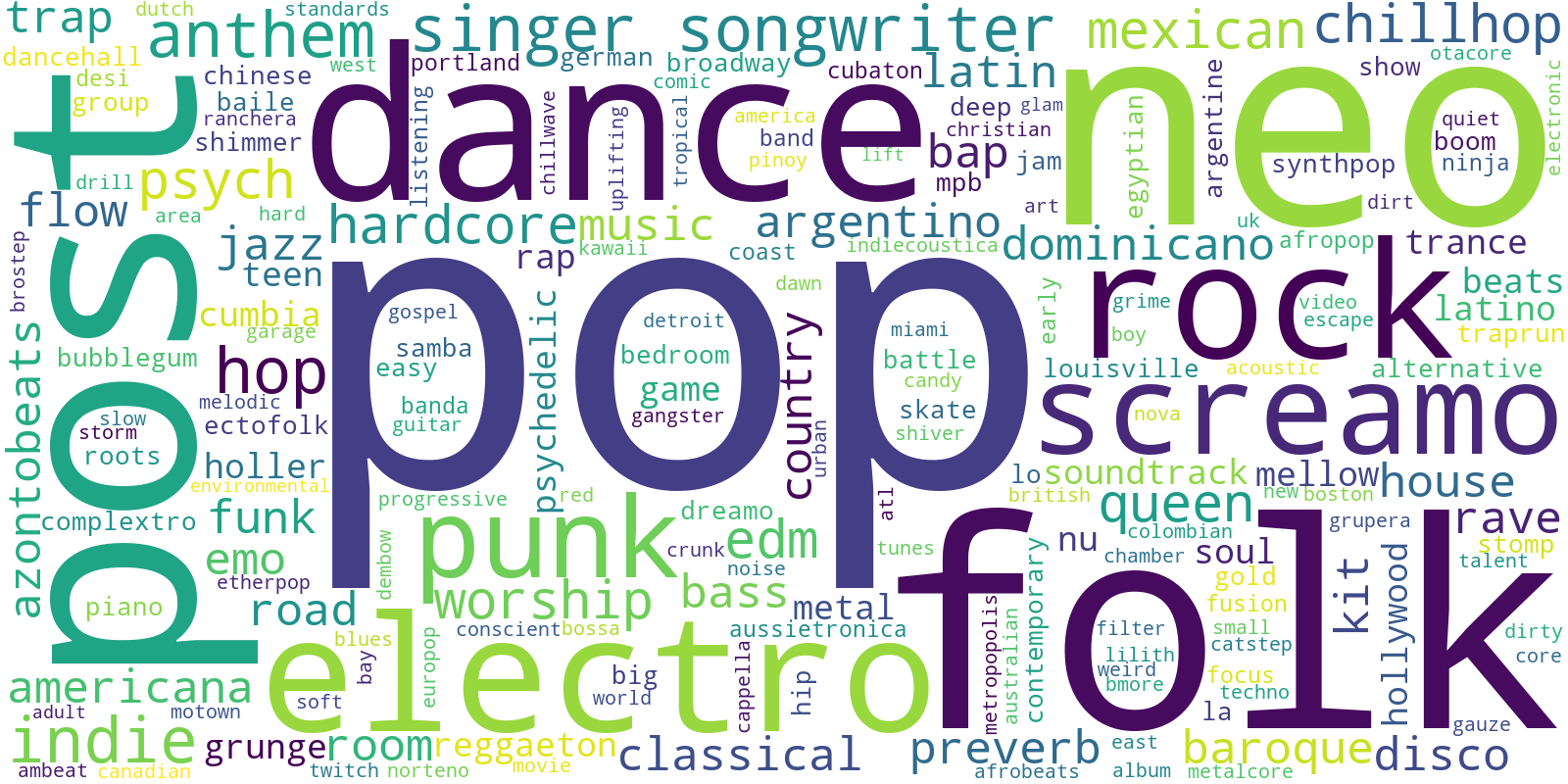
To explore the genres more, we can transform the genres tags into cloud of words and investigate their frequencies.
Python code
"""
- generate a column of words counts dictionaries
- create new frame with columns as separate tags

"""

df['words_count'] = df.genres_all.apply(lambda x: Counter(x.split(' ')))
gen_table=pd.DataFrame(df.words_count.values.tolist())
gen_table[np.isnan(gen_table)] = 0


"""
- for each review perform transformation into string type
- generate the cloud of words using Wordcloud() module

"""

# create wordcloud object with gen_table as an argument
wordcloud = WordCloud(background_color='white', width=1600, height=800).generate(' '.join(gen_table))
# plot as a figure
plt.figure(figsize=(12,8))

plt.imshow(wordcloud, interpolation = 'bilinear')
plt.axis('off')
plt.tight_layout(pad=0)
plt.show()
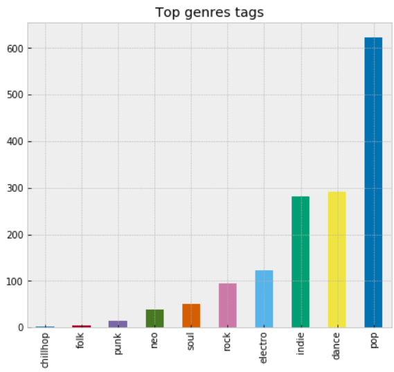
Finally, let's count some of the most popular tags from WordCloud and represent using bar chart.
Python code
"""
- initialize the list of genres we are interested in
- apply sorting to display ascending order

"""

list_g = ['pop', 'folk', 'neo', 'electro', 'punk', 'dance', 'rock', 'soul', 'indie', 'chillhop']

rcParams['figure.figsize'] = 7, 6

gen_table[list_g].sum().sort_values(ascending=True).plot(kind='bar')
plt.title('Top genres tags')