Taxi Fare Predictions - Google BigQuery Data (Part 2)

Model preparation

On this stage we are working on regression problem to build a predictive model for taxi fares.
To derive percise predictions we will take different algorithms into consideration:

1. Multiple regresssion with regularization component(L1/L2);
2. Random forest model;
3. XGBoost model.

1.1 Linear model without regularization

We start with spliting data on train-validation and test. Using 10% of data as test sample we train basic linear model and estimate performance metrics - MAE (mean absolute error) and RMSE (root squared error) on test. To simplify our code on further steps we will write a function to estimate metrics for different models.

Python code

"""
- perform train_test_split() mudule for data split
- separate the  relevant features list and target as an output 

"""
train_valid_data, test_data = train_test_split(data, test_size=0.1)

features=['dropoff_longitude','dropoff_latitude', 'pickup_longitude', 'pickup_latitude', 
        'distance_trip', 'diff', 'passenger_count', 'dropoff_month', 'dropoff_day', 'dropoff_hour',
        'pickup_month', 'pickup_day', 'pickup_hour']
output='fare_amount'

"""
- define the function to compute errors 
- print the result on test data

"""

def compute_error(predictions, true_values):
   resid=true_values-predictions
   rss = sum(resid*resid)
   # computing root mean absolute error 
   mae_true=sum(abs(resid))/len(predictions)
   # computing root mean squared error 
   mse_true=rss/len(resid)
   rmse_true=np.sqrt(mse_true)
   
   print "RMSE on test equals "+ "{:.{}f}".format( rmse_true, 2 )
   print "MAE on test  equals "+"{:.{}f}".format( mae_true, 2 )  

Now we are ready to train base regression model on train_valid_data and evaluate performace on test.

Python code

"""
- create a linear regression object
- fit with train-validation data
- make predictions on test

"""
linear=LinearRegression(normalize=True)
linear.fit(train_valid_data[features], train_valid_data[output])
predictions=linear.predict(test_data[features])
compute_error(predictions, test_data[output])

RMSE on test equals 3.09
MAE on test  equals 2.31

The results above represent performance for unregularized model. Let's check the possible improvement with regularization parameter added.

1.2 Ridge regression

Next we will use train-validation data to build regression model with L2 regularization, performing k-folds cross validation to tune regularization parameter. For each fold we train a model and compute mean squared and root mean squared errors to find mean across folds. Besides we are going to visualize the mean absolute error change with respect of penalty parameter value.

Display split per folds:

Python code

"""
- use number of folds k=10  
- display folds boundaries for train-validation data

"""

n = len(train_valid_data) # will use entire frame
k=10
# print boundaries for each fold 
for fold in range(k):
   start = (n*fold)/k 
   end = (n*(fold+1))/k-1
   print fold, (start, end)

0 (0, 153424)
1 (153425, 306850)
2 (306851, 460276)
3 (460277, 613701)
4 (613702, 767127)
5 (767128, 920553)
6 (920554, 1073978)
7 (1073979, 1227404)
8 (1227405, 1380830)
9 (1380831, 1534256)

Train Ridge regression for each parameter from list and compute metrics means.

Python code

"""
- initialize the list of penalty values and starting points: split on train/validation, 
compute error for each fold, sum it up and estimate the average error for particular penalty 

"""

l2_penalty=[1e-17, 1e-12, 1e-06, 0.001, 0.01, 1, 2]
mae_sum = 0
rmse_sum = 0
mae_penalty=[]
# iterate through penalty values, create Ridge object 
for alpha in l2_penalty:
   ridge=linear_model.Ridge(alpha=alpha, normalize=True)
   for i in xrange(k):
       start=(n*i)/k
       end=(n*(i+1))/k-1
       valid=train_valid_data[start:end+1]
       training=train_valid_data[0:start].append(train_valid_data[end+1:n])
       # fitting model, making predictions 
       ridge.fit(training[features], training[output])
       predictions=ridge.predict(valid[features])
       resid=valid[output]-predictions
       # computing rss
       fold_rss = sum(resid*resid)
       # computing mean absolute error 
       fold_mae=sum(abs(resid))/len(predictions)
       mae_sum+=fold_mae
       # computing root mean squared error 
       fold_mse=fold_rss/len(resid)
       fold_rmse=np.sqrt(fold_mse)
       rmse_sum+=fold_rmse
   # estimate validation errors for each alpha 
   val_mae = mae_sum/k
   val_rmse = rmse_sum/k 
   mae_penalty.append(val_mae)
   print "RMSE for alpha=" +str(alpha)+' equals '+ "{:.{}f}".format( val_rmse, 2 )
   print "MAE for alpha="+str(alpha)+' equals '+"{:.{}f}".format( val_mae, 2 )

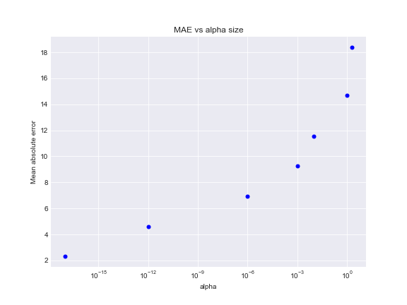
RMSE for alpha=1e-17 equals 3.08
MAE for alpha=1e-17 equals 2.31
RMSE for alpha=1e-12 equals 6.16
MAE for alpha=1e-12 equals 4.62
RMSE for alpha=1e-06 equals 9.25
MAE for alpha=1e-06 equals 6.93
RMSE for alpha=0.001 equals 12.33
MAE for alpha=0.001 equals 9.25
RMSE for alpha=0.01 equals 15.41
MAE for alpha=0.01 equals 11.56
RMSE for alpha=1 equals 19.38
MAE for alpha=1 equals 14.71
RMSE for alpha=2 equals 23.97
MAE for alpha=2 equals 18.40

Plot below presents the mean absolute error increases with respect of penalty rate growth. The best choice will be to fit model with a small alpha value to avoid underfitting.

Python code

fig, ax = plt.subplots(figsize=(8,6))
# plot log-scale x-axis  for alpha values 
plt.plot(l2_penalty, mae_penalty,'b.', markersize=10)
plt.xscale('log')
ax.set_title('MAE vs alpha size')
ax.set_xlabel('alpha')
ax.set_ylabel('Mean absolute error')

Make predictions on test data with alpha=1e-17, compute metrics. Since alpha value is quite small, penalization effect will be insignificant and ridge solution will have the same performance as in case of least squares method.

Python code

"""
- fitting model with best penalty size 
- compute metrics on test

"""

# fitting model with best penaty size
# making predictions on test data

ridge_best=linear_model.Ridge(alpha=1e-17, normalize=True)
ridge_best.fit(train_valid_data[features], train_valid_data[output])
predictions=ridge_best.predict(test_data[features])
compute_error(predictions, test_data[output])

RMSE on test equals 3.09
MAE on test  equals 2.31

Let's dispay coefficients of trained models with related features.

Python code

print 'Coefficients for Ridge model:'
list(zip(features, ridge_best.coef_))

Coefficients for Ridge model:
[('dropoff_longitude', 13.760057467731182),
('dropoff_latitude', -1.9637103194625796),
('pickup_longitude', 18.359401690053996),
('pickup_latitude', 7.8960641296256044),
('distance_trip', 1.2034294882452077),
('diff', 0.005993982157018705),
('passenger_count', 0.012286631700869122),
('dropoff_month', -0.062067925417318745),
('dropoff_day', 0.0005984279860302647),
('dropoff_hour', -0.013282399216881468),
('pickup_month', 0.05996505422940662),
('pickup_day', 0.00020709144512874323),
('pickup_hour', -0.029342367697220418)]

Below we see insignificant difference in coefficients values between base model and model with small alpha regularization.

Python code

print 'Coefficients for Linear model:'
list(zip(features, linear.coef_))

[('dropoff_longitude', 13.760057467731158),
('dropoff_latitude', -1.9637103194626524),
('pickup_longitude', 18.35940169005395),
('pickup_latitude', 7.896064129625596),
('distance_trip', 1.2034294882452132),
('diff', 0.005993982157018712),
('passenger_count', 0.012286631700870652),
('dropoff_month', -0.062067925414981726),
('dropoff_day', 0.000598427986083889),
('dropoff_hour', -0.01328239921687862),
('pickup_month', 0.05996505422707346),
('pickup_day', 0.00020709144507718473),
('pickup_hour', -0.029342367697224047)]

1.3 Lasso regression

Perform the same process for Lasso regression, tuning the parameters with 10-folds cross-validation.

Python code

# use higher alpha values for L1 regularization 
l1_penalty = [1e-7, 1e-5, 1e-3, 1e-2, 1e-1, 1, 5]
n = len(train_valid_data)
k=10
mae_sum=0
rmse_sum=0
mae_penalty=[]

"""
- train Lasso model, specifying maximum iteration=1e5
- split by train and valid data sets, compute validation metrics

"""

for alpha in l1_penalty:
   lasso=Lasso(alpha=alpha,normalize=True, max_iter=1e5)
   for i in xrange(k):
       start=(n*i)/k
       end=(n*(i+1))/k-1
       valid=train_valid_data[start:end+1]
       training=train_valid_data[0:start].append(train_valid_data[end+1:n])
       # fitting model, making predictions 
       lasso.fit(training[features], training[output])
       predictions=lasso.predict(valid[features])
       resid=valid[output]-predictions
       # computing rss
       fold_rss = sum(resid*resid)
       # computing mean absolute error 
       fold_mae=sum(abs(resid))/len(predictions)
       mae_sum+=fold_mae
       # computing root mean squared error 
       fold_mse=fold_rss/len(resid)
       fold_rmse=np.sqrt(fold_mse)
       rmse_sum+=fold_rmse
   val_mae = mae_sum/k
   val_rmse = rmse_sum/k 
   mae_penalty.append(val_mae)
   print "RMSE for alpha=" +str(alpha)+' equals '+ "{:.{}f}".format( val_rmse, 2 )
   print "MAE for alpha="+str(alpha)+' equals '+"{:.{}f}".format( val_mae, 2 )

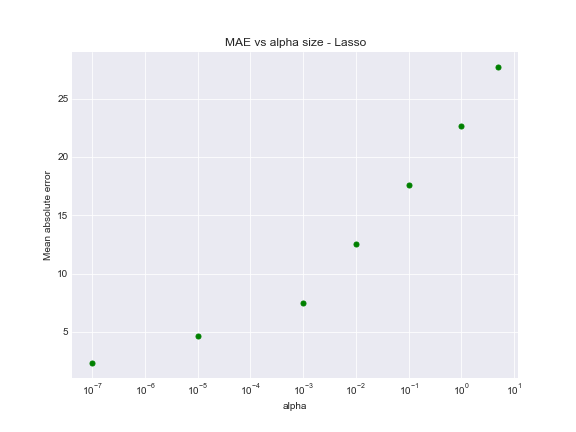
RMSE for alpha=1e-07 equals 3.08
MAE for alpha=1e-07 equals 2.31
RMSE for alpha=1e-05 equals 6.16
MAE for alpha=1e-05 equals 4.63
RMSE for alpha=0.001 equals 9.83
MAE for alpha=0.001 equals 7.50
RMSE for alpha=0.01 equals 16.01
MAE for alpha=0.01 equals 12.56
RMSE for alpha=0.1 equals 22.19
MAE for alpha=0.1 equals 17.62
RMSE for alpha=1 equals 28.37
MAE for alpha=1 equals 22.68
RMSE for alpha=5 equals 34.55
MAE for alpha=5 equals 27.74

L1 had considerable effect on model performance, adding sum of the absolute value of the coefficients as a penalty term.

Python code

fig, ax = plt.subplots(figsize=(8,6))
plt.plot(l1_penalty, mae_penalty,'g.', markersize=10)
plt.xscale('log')
ax.set_title('MAE vs alpha size - Lasso')
ax.set_xlabel('alpha')
ax.set_ylabel('Mean absolute error')

Regularized L1 model with small alpha performs in the same way as base model.

RMSE on test equals 3.09
MAE on test  equals 2.31

Hence we observe the same fact of underfitting for Lasso regression, hence the better approach is to process with a small regularization term.

2.1 Random Forest model

To train higher performance models for predictions, we contunue with applying non-parametric algorithms. In this case we will learn functional relationships from data, not making strong assumptions about function's form.

Strating with Randon Forest regression algorithm, build a model with specified trees and minimum leaf samples parameters.

Python code

"""
- n_estimators=100 - computation using 100 trees in model
- samples in leaf node=5
- make predictions and compute same metrics

"""
rf_reg = RandomForestRegressor(random_state = 123, n_estimators=100, n_jobs=-1, min_samples_leaf =5)
rf_reg.fit(train_valid_data[features], train_valid_data[output])

predictions=rf_reg.predict(test_data[features])
compute_error(predictions, test_data[output])

RMSE on test equals 2.08
MAE on test  equals 1.42

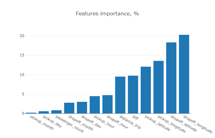
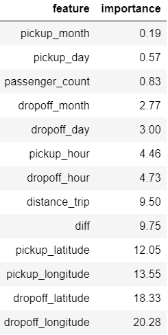
To learn the features importance of the trained model, we are able to call feature_importances_ function below:

Python code

"""
- use argsort function() to sort per importance rate
- plot importance rate wih related features

"""
def display_importance(model):
   importance_list=[]
   feat_list=[]
   importance = model.feature_importances_
   feature_indices = importance.argsort()
   for index in feature_indices: 
       importance_list.append(round(importance[index] *100.0,2))
       feat_list.append(features[index])
   imp=pd.DataFrame({'feature': feat_list, 'importance': importance_list})
   data = [go.Bar(
           x=imp['feature'],
           y=imp['importance'])
      ]
   layout = go.Layout(title='Features importance, %')
   fig = dict(data=data, layout=layout)
   iplot(fig)
   return imp
   
# apply function to display results
display_importance(rf_reg)

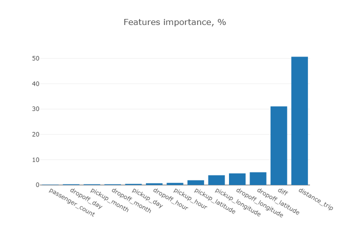
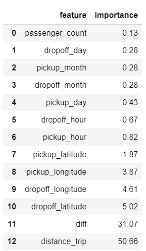
Seems that trip distance and trip duration provide the highest importance contribution to overall performance, while the features like passenger count and time attributes shown unsignificant.

2.2 XGBoost model

Finally, we apply Gradient boosing algorithm to perform desicion trees ensemble approach and present the features importance using function defined previously.

Python code

xgboost_reg = xgb.XGBRegressor(n_estimators=100, learning_rate=0.07, eta=1, 
                              eval_metric = 'rmse', max_depth=10)
xgboost_reg.fit(train_valid_data[features], train_valid_data[output])
predictions=xgboost_reg.predict(test_data[features])
compute_error(predictions, test_data[output])
# apply function to display results for XGboost
display_importance(xgboost_reg)

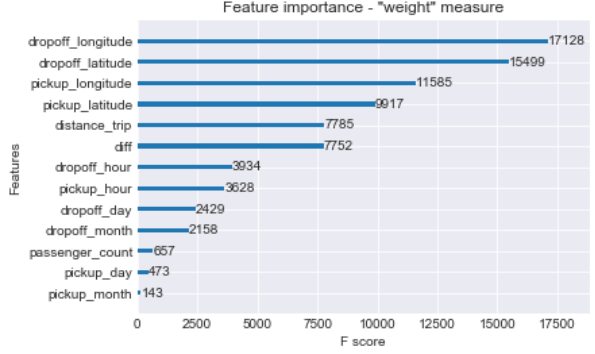
With XGboost model fitting dropoff coordinte features dominate the others in contrast with random forest model. However, we assume the different options for XGboost to measure features importance.
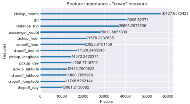
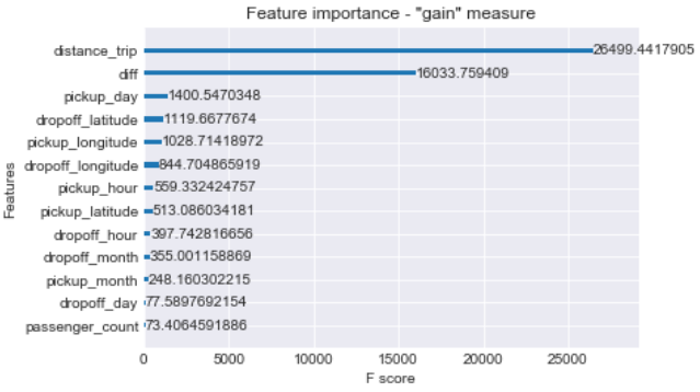
The chart below represents different order of features importance in terms of type:

• "weight": by number of times feature used to split data across the trees;
• "cover": number of times feature used to split data across the trees, but wighted by training data points;
• "gain": by average training loss reduction of feature use for split.

The best importance measure choice generally relies on model consistency and ability to miinimize the error.

Python code

# plot importance based on 'weight' measure
xgb.plot_importance(xgboost_reg, importance_type='weight')
plt.title('Feature importance - "weight" measure')
# based on 'cover' measure
xgb.plot_importance(xgboost_reg, importance_type='cover')
plt.title('Feature importance - "cover" measure')
# based on 'gain' measure
xgb.plot_importance(xgboost_reg, importance_type='gain')
plt.title('Feature importance - "gain" measure')

Results and models comparison

Python code

results=pd.DataFrame({'model':['Linear regression', 'Ridge regression', 'Lasso regression',
                             'Random Forest', 'XGBoost regressor'],
                    'RMSE':[3.09, 3.09, 3.09, 2.05, 2.05],
                    'MAE':[2.31, 2.31, 2.31, 1.42, 1.46]})
trace0 = go.Table(
 header = dict(
   values = list(results.columns[::-1]),
   line = dict(color = '#506784'),
   fill = dict(color =  '#b8b894'),
   align = ['left','center', 'center'],
   font = dict(color = 'white', size = 12)
 ),
 cells = dict(
   values = [results['model'], results['RMSE'], results['MAE'] 
            ],
   line = dict(color = '#506784'),
   fill = dict(color =  '#e0e0d1'),
   align = ['left', 'center', 'center'],
   font = dict(color = '#506784', size = 11)
   ))

data = [trace0]
iplot(data)

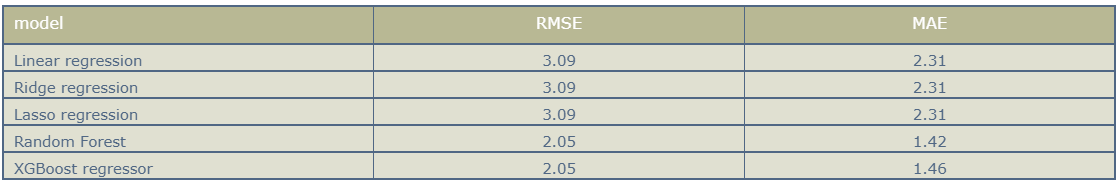
In terms of RMSE measurement we see Random Forest and XGBoost models obtain the same results and reduce the fare of amount error prediction to 2.05.

However, the further tunning models on search grid potentially can lead even to a higher result. Estimated RMSE with linear model fitting approaches 3.09 value and gives practically the same result with small regularization parameter.

Besides, in terms of "bias-variance" tradeoff it's worth mentioning the difference between RF and XGBoost approches. While boosted trees tend to reduce bias and decreasing a generalization error, combining weak high-biased learners, RF in opposite, grows low-biased trees and minimizes the error by variance reduction.