Volvo sales data - Explanatory data analysis and Time series modelling

Background

Vovlo Car Group finalized the sales results of 2018 year in official release and hit the global record of 600.000 sales.

The major contribution to overall sales growth was driven by China (14.1%) and US (20.6%).
In comparison with December'17 we see the slight demand slowdown in Europe region (-1.3%) and US (-8.8%). However, total December volumes represent sustainable growth year over year.

To effectively predict auto sales and improve Volvo Group competitiveness we will analyze the monthly data and, revealing seasonal flactuations derive predictions powered by neural network.

Main goal

Analyze monthly sales data and build predictive model according to listed steps:

• Explore sales data and establish ETL into Google BigQuery;
• Perform Explanatory data analysis of time series;
• Model preparation and evaluating;
• Provide recommendataions for further improvement.

Entire process can be illustrated by diagram:

Data

Data we will use for this project is published on Volvo Car Group official website and contains:

• monthly sales volumes;
• auto model;
• respected time period - month, year.

To be consistant we will add respected time period column in following format: "YYYY-MM-DD".

Data preprocessing

Step 1: Primary data cleaning

Initial CSV dataset is availbale in repository via the link We start with data transformation into suitable for analysis format:

• Convert sales amount column in "int" format;
• Retrieve month and year stamps from date columns;
• Write resulted columns into .csv file.

Python code

"""
- import librariies for data manipulation  
- split date into month/year
- write dataframe into new csv 

"""

import pandas as pd
import datetime as dt
import warnings
warnings.filterwarnings("ignore")

# reading csv file
df= pd.read_csv('sales.csv', sep=';', encoding='utf-8')
df.drop('Unnamed: 5', axis=1, inplace=True)
# convert to str and numeric
df['sales'] = df['sales'].astype('str')
df['sales']=pd.to_numeric(df['sales'])
# date convertion
df['date'] = df['date'].apply(lambda x: dt.datetime.strptime(x, '%Y-%m-%d'))
df['date_year'] = [x.strftime('%Y')for x in df['date']]
df['date_month'] = [x.strftime('%m')for x in df['date']]
# reading into csv
df=df[['model', 'date', 'sales', 'date_year', 'date_month']]
df.to_csv('sales_full.csv', encoding='utf-8')

Step 2: Store data with Google Cloud Storage

On this stage we upload data into Cloud Storage to establish data transfer over all Google services. Since the files are uploaded on GitHub we can use Git to clone repository and store entire folder. Using Google Shell type following command:

$ git clone https://github.com/MakarovArtyom/side_projects.git
$ cd side_projects/volvo_data
$ head sales_all.csv

Explore the .csv in Output:

,model,date,sales,date_year,date_month0,S60 CC,2018-12-31,87,2018,121,S60 II,2018-12-31,961,2018,122,S60L,2018-12-31,1314,2018,123,S80 II,2018-12-31,0,2018,124,S90,2018-12-31,5108,2018,125,V40,2018-12-31,5121,2018,126,V40 CC,2018-12-31,1591,2018,127,V60,2018-12-31,524,2018,128,V60 CC,2018-12-31,249,2018,12

Next we need to create a "bucket" and store the files (additionally we create folder 'sql'):

$ gsutil cp cloudsql/* gs://<BUCKET-NAME>/sql/ 

Step 3: Upload into Google BigQuery

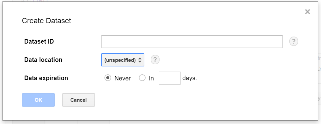
On this stage we will load .csv file into BigQuery, create a table and query data. Start with dataset creation:

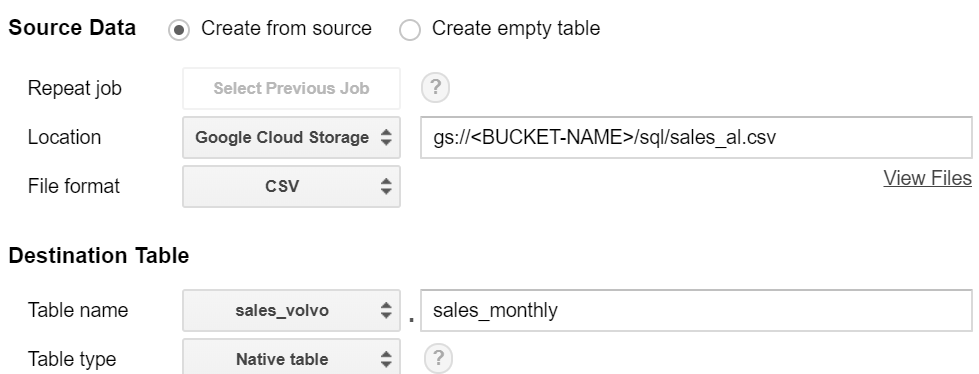
Continue with creating a table, we load sales_all.csv from storage, specifiyng the name - "sales_monthly".

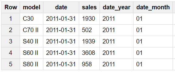
Finally, use SQL syntax to query a table:

SELECT model, date, sales, date_year, date_month
FROM
 [prredictions:sales_volvo.sales_monthly]
LIMIT
 1600

Loading dataset to Notebook

Now we are ready to import and analyze time series in Jupyter notebook. We will use Plotly to visualize the data, Pandas package for data manupulation and Keras for model building.

Python code

"""
- import Plotly modules for interactive data visualization 
- connect to plot inside notebook
"""

from plotly.offline import download_plotlyjs, init_notebook_mode, plot, iplot
import plotly.plotly as py
import plotly.graph_objs as go
import colorlover as cl
import cufflinks as cf
init_notebook_mode(connected=True)

# data manipulation libraries
import pandas as pd  
from pandas.io import gbq # retrieve google big query data
import numpy as np           
import matplotlib.pyplot as plt 
%pylab inline
plt.style.use('seaborn-whitegrid')

# will ignore the warnings
import warnings                 
warnings.filterwarnings("ignore")

# keras to build LSTM network 
import math
from keras.models import Sequential
from keras.layers import Dense
from keras.layers import LSTM
from sklearn.preprocessing import MinMaxScaler
from sklearn.metrics import mean_squared_error

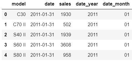
Once we're done we can start to load and explore dataset.

sql = """
   SELECT *
   FROM `sales_volvo.sales_monthly`
   LIMIT 1600
# Run a Standard SQL query with the project set explicitly
project_id = 'prredictions'
sales = pd.read_gbq(sql, project_id=project_id, dialect='standard')
sales.head()
"""

Explonatory analysis

Starting with listing down a number of variables affecting amount of sales:

1. Sales per month - the sales amount can differ depends on month;
2. Sales per year - the sales amount can flactuate depending on year;
3. Sales per model - particular Volvo model represents differnet sales amount in time.

Time period effect

On the graph we see the tendency of average sales amount reaches its peak at the last month of each quarter.

Besides, we see the positive trend per year with the highest total sales results in 2018.

Volvo sales per model

Then we can estimate the mean sales per model and get the top performers over the years.

Python code

"""
- choose the color scale - will use different colors for models
- use cufflinks package to plot from dataframe
"""
color_scale = ['rgb(102, 102, 255)', 'rgb(102, 153, 255)',
                    'rgb(102, 102, 255)', 'rgb(102, 0, 255)', 
                    'rgb(153, 153, 255)', 'rgb(51, 153, 255)', 
                    'rgb(0, 153, 255)', 'rgb(0, 102, 204)', 
                    'rgb(0, 153, 204)',
                    'rgb(0, 102, 153)', 'rgb(51, 102, 153)', 
                    'rgb(0, 51, 153)','rgb(51, 51, 153)', 
                    'rgb(102, 102, 153)', 'rgb(102, 0, 255)',
                    'rgb(153, 51, 255)', 'rgb(102, 0, 102)', 
                    'rgb(204, 0, 153)', 'rgb(153, 0, 153)', 
                    'rgb(153, 51, 102)', 'rgb(117, 87, 87)',
                    'rgb(112, 92, 92)', 'rgb(87, 87, 117)', 
                    'rgb(117, 94, 87)','rgb(179, 152, 152)', 'rgb(88, 65, 65)']
cf.set_config_file(offline=True, world_readable=True, theme='white')

sales_model.iplot(kind='bubble', x='model', y='sales', size='sales', 
                 title = 'Sales Average per Model',
            xTitle='model', yTitle='sales amount',
            filename='cufflinks/simple-bubble-chart', colors=color_scale)

On average the highest selling auto models are XC60, XC60 II and XC90 II - we can investigate the time series of these models more presicely and plot on chart. XC60 II represents the rocket growth starting from end of 2017 and keeps trend within 2018. However, the sales of old version XC60 decrease along with sustainable flactuations of XC90 II.

Python code

"""
- plot scatter for 3 top performed models
- add rangeslider to navigate between periods
"""
pivot=pd.pivot_table(sales, values='sales', index=['date'], columns=['model'], aggfunc=np.sum)
pivot.fillna(0, inplace=True)
trace_1 = go.Scatter(
   x=pivot.index,
   y=pivot['XC60'],
   name = "model: XC60",
   line = dict(color = '#dd870f'),
   opacity = 1)

trace_2 = go.Scatter(
   x=pivot.index,
   y=pivot['XC60 II'],
   name = "model: XC60 II",
   line = dict(color = '#7F7F7F'),
   opacity = 1)


trace_3 = go.Scatter(
   x=pivot.index,
   y=pivot['XC90 II'],
   name = "model: XC90 II",
   line = dict(color = '#0b7782'),
   opacity = 1)

data = [trace_1,trace_2, trace_3]

layout = dict(
   title='Top 3 High-Performed Models',
   xaxis=dict(
       rangeselector=dict(
           buttons=list([
               dict(count=1,
                    label='6m',
                    step='month',
                    stepmode='backward'),
               dict(count=6,
                    label='12m',
                    step='month',
                    stepmode='backward'),
               dict(step='all')
           ])
       ),
       rangeslider=dict(
           visible = True
       ),
       type='date'
   )
)

fig = dict(data=data, layout=layout)
iplot(fig)

Inspect volatility

Let's add moving average line for entire time series to see how this method approxiamtes true values. Choose window size equals 3.

Python code

""" 
- group entire sales by date column
- use .rolling() function to estimate mean 
- add resulted column to dataframe 
"""
data_moving=sales.groupby('date')['sales'].sum().to_frame()

data_moving['3_moving_av']= data_moving['sales'].rolling(window=3, min_periods=0).mean()

trace_1 = go.Scatter(
   x=data_moving.index,
   y=data_moving['sales'],
   name = "sales amount",
   line = dict(color = '#dd870f'),
   opacity = 1)

trace_2 = go.Scatter(
   x=data_moving.index,
   y=data_moving['10_moving_av'],
   name = "moving-average",
   line = dict(color = '#7F7F7F'),
   opacity = 1)

data = [trace_1,trace_2]

layout = dict(
   title='Moving average for sales amount')

fig = dict(data=data, layout=layout)
iplot(fig)

We see the moving average method barely predicts the consequent values. The volatility of series is quite high and process is characterized by systematic cycles. Additionally we are able to apply differencing and prepare stationarity test based on Dickey-Fuller criteria.

Python code

"""
- perfrom differencing of 7 order
- use .adfuller() function from stattools module to estimate criterion
"""
data_diff=sales.groupby('date')['sales'].sum().to_frame()
data_diff['sales_diff'] = data_diff['sales'].diff(7)
trace = go.Scatter(
   x=data_diff.index,
   y=data_diff['sales_diff'],
   name = "diff_sales",
   line = dict(color = '#dd870f'),
   opacity = 1)

data = [trace]

layout = dict(
   title='Sales series with 7 order differencing')

fig = dict(data=data, layout=layout)
iplot(fig)
print("Dickey-Fuller criteria: p=%f" % sm.tsa.stattools.adfuller(data_diff['sales_diff'][7:])[1])

Dickey-Fuller criteria: p=0.485103

Dickey-Fuller criteria proves the resulted series can not be categorized as stationary.

Time series modelling

Time series prediction problem is a difficult type of modeling problem. To reach a maximum results we need use a method that handles sequently dependent values. One of the powerful kind of recurrent neural networks that solves time-series problem is Long Short-Term Memory network (LSTM).

It has a chain structure, consisted of cells and gates, that are able to remove or add information. On the schema below we see three gates where sigmoid layer regulates the cell state and presents an output of between 0 (do not let information through) and 1 (through the entire piece of information).

By Guillaume Chevalier - Own work, CC BY 4.0, Link

Detailed LSTM components are described in original paper.

Stage 1: Pre-processing

For our project we will use Keras deep learning library to train LSTM network.
First, preprare the dataset: we need to normalize the data to [0;1] range to prepare the scale for activation function.

Python code

'''
- retrieve series values with .values
- use MinMaxScaler() from scikit-learn preprocessing module

'''

data=sales.groupby('date')['sales'].sum().to_frame()
numpy.random.seed(7)
data = data.values
data = data.astype('float32')
scaler = MinMaxScaler(feature_range=(0, 1))
data = scaler.fit_transform(data)

Then we prepare train/test split for our data. We will use 65/35 proportion to train and evaluate model.

Python code

# split into train and test sets
train_size  = int(len(data) * 0.65)
test_size = len(data) - train_size
train, test = data[0:train_size,:], data[train_size:len(data),:]
print(len(train), len(test))

62 34

Continue with recreating a new dataset with two columns from existing data, that consists of sales in $t$ period and $t+1$ time period, that supposed to be predicted. Assume lag=7 as a number of previous time periods to use as an input.

Python code

  
"""
- start with creating an empty list for both data and target 
- reshape values for t period and t+1 for X and y (start with lag-1 to put first value in dataset)

"""

def reshape_dataset(dataset, lag):
    X=list()
    y=list()

    for i in range(len(dataset)-lag-1):
        a = dataset[i:(i+lag), 0]
        X.append(a)
        y.append(dataset[i + lag, 0])
    return np.array(X), np.array(y)

lag=7
train_X, train_y = reshape_dataset(train, lag)
test_X, test_y = reshape_dataset(test, lag)

Last step for preparation is to create data structure required for LSTM network in form of (#samples, #time steps, #features).

Python code

train_X = np.reshape(train_X, (train_X.shape[0], 1, train_X.shape[1]))
test_X = np.reshape(test_X, (test_X.shape[0], 1, test_X.shape[1]))

Stage 2: Model building

We assume network has a one-input layer with lag=7, memory blocks=4 and mean squared error as a loss function. Besides, the single output will be produced by dense layer.

Python code

# create and fit the LSTM network
model = Sequential()
model.add(LSTM(4, input_shape=(1, lag)))
model.add(Dense(1, activation = 'linear'))
model.compile(loss='mean_squared_error', optimizer='adam')
model.fit(train_X, train_y, epochs=90, batch_size=1, verbose=2)

....
Epoch 85/90
- 0s - loss: 0.0102
Epoch 86/90
- 0s - loss: 0.0099
Epoch 87/90
- 0s - loss: 0.0097
Epoch 88/90
- 0s - loss: 0.0098
Epoch 89/90
- 0s - loss: 0.0097
Epoch 90/90
- 0s - loss: 0.0097

Stage 3: Model evaluation

Perform inverse transformation and evaluate model results.

Python code

"""
- make predictions on train and test samples
- use inverse_transform() function to perform inverse transformation
- calculate metrics on train/test
"""

predict_train = model.predict(train_X)
predict_test = model.predict(test_X)

predict_train = scaler.inverse_transform(predict_train)
train_y = scaler.inverse_transform([train_y])
predict_test = scaler.inverse_transform(predict_test)
test_y = scaler.inverse_transform([test_y])

mse_train = math.sqrt(mean_squared_error(train_y[0], predict_train[:,0]))
print('RMSE on train: %.2f' % (mse_train))
mse_test = math.sqrt(mean_squared_error(test_y[0], predict_test[:,0]))
print('RMSE on test: %.2f' % (mse_test))

RMSE on train: 3709.17
RMSE on test: 5044.35

After the metrics are calculated we need to visualize the predictions with respect of true values to see check the underestimated/overestimated areas.

Python code

"""
- shift train/test predictions for plotting
- write to a dataframe with actual values
"""
train_pred = numpy.empty_like(data)
train_pred[:, :] = numpy.nan
train_pred[lag:len(predict_train)+lag, :] = predict_train

test_pred = numpy.empty_like(data)
test_pred[:, :] = numpy.nan
test_pred[len(predict_train)+(lag*2)+1:len(data)-1, :] = predict_test
# add date column to values 
res=pd.DataFrame(data=list(sales.groupby('date')['sales'].sum().to_frame()['sales']))
res['date']=sales.groupby('date')['sales'].sum().to_frame().index
res=res.rename(columns={0: 'true_values'})
res['train_predictions']=train_pred # train_pred
res['test_predictions']=test_pred # test_pred

Predictions represent the shape of actual series, repeating the seasonal behaviour of monthly sales.

Python code

trace_1 = go.Scatter(
   x=res.date,
   y=res['true_values'],
   name = "Actual sales",
   line = dict(color = '#dd870f'),
   opacity = 1)

trace_2 = go.Scatter(
   x=res.date[7:train_size-1],
   y=res['train_predictions'][7:train_size-1],
   name = "Train predictions",
   line = dict(color = '#7F7F7F'),
   opacity = 1)


trace_3 = go.Scatter(
   x=res.date[69:95],
   y=res['test_predictions'][69:95],
   name = "Test predictions",
   line = dict(color = '#0b7782'),
   opacity = 1)

data = [trace_1,trace_2, trace_3]

layout = dict(
   title='Sales predictions - LSTM model')


fig = dict(data=data, layout=layout)
iplot(fig)

Inspecting predictions on train sample we see the model performs quite well in general, replicating the shape of actual values (for instance, high precision in 2015 year).

However, we assume that model does not cover the sharp peaks, underestimating predictions in highly-selling periods (March'14 or December'15).

The similar tendency is observed on test sample below.

• Overestimating can cause too positive prediction and wrong beliefs, that often leads to high targets setting and production costs increase.
  
• Underestimating in opposite, can lead to wrongly negative market outlook.

Futher Improvement

There are possible improvements we would merits mention for problem of sales prediction.

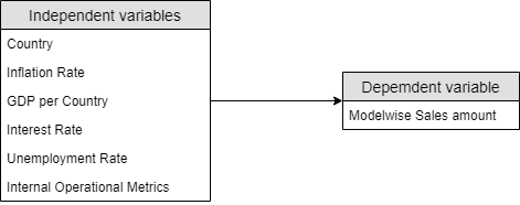
1. Multivariate model preparation.

One of the reasonable improvement, especially in terms of long-term forecasting will be including multiple variables in model, such as:

1. Country - exploration of local market features;
2. GDP - propose the hypothesis of a positive relationship between GDP and sales;
3. Inflation rate - IR tends to show negative correlation with sales;
4. Unemployment rate - along with IR, unemployment rate can negatively effect on sales amount;
5. Interest rate - negative impact on consumer power.

Model-wise predictions are highly important for precise analysis: it's worth more tuning parameters for multiple smaller models than construct one complex.

Additionaly, the quality of domestic manufactured cars matters: consumers of different countries tend to purchase imported cars if they believe in higher quality.

2. Existing model tuning

The current predictive model can be improved with both dataset enlarging and hyperparameters tuning. In case of LSTM model this can be related to:

1. Training epochs value;
2. Memory blocks;
3. Window (lag) value - tune the number of "look back" time periods;
4. Stochastic optimizer choosing.